PSEB Solutions for Class 9 Computer Science Chapter 4 MS Excel Part-II

03/29/2023 Ajit kumar 144 Views 0 Comments

PSEB 9th Class Computer Solutions Chapter 4 MS Excel Part-II

INTRODUCTION

Formatting tools are very useful in MS Excel. Data can be formatted as per requirement using those tools.

FORMATTING IN MS EXCEL

Excel sheets are very difficult to understand without formatting. Formatted data and cells can be useful to get attention to specific parts of data. It make data more visually appealing and easier to understand. There are many tools in Excel for formatting. These can be used for formatting text and cells. These tools can change the colour and style, alignment and apply special formatting to numbers and dates.

Changing the Text Styles

Excel offers lots of different options to change the text styles. Some of these are:

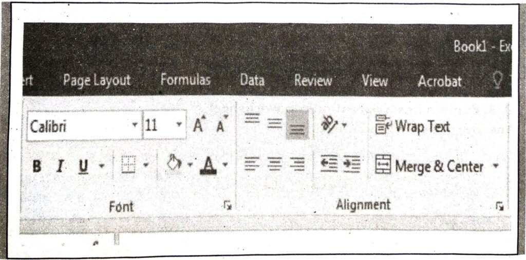
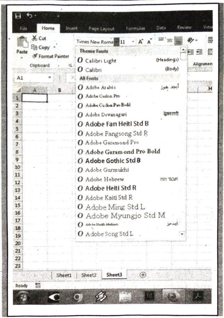
1. Font: A Font is a style of text. It can be changed. Some basic fonts are Times, Arial, Times new Roman, AnmolLipi etc.

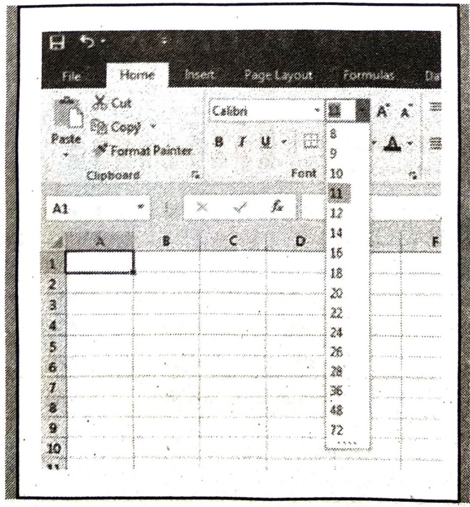
2. Size: This option of text style increases or decreases the size of text. Contents in different sizes in a single worksheet make it more effective.

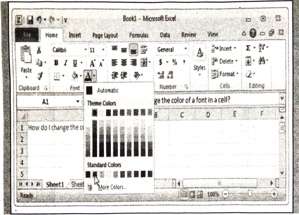
3. Font Colour: The colour of contents can be changed in Excel. There is a wide range of colours available for Foreground of text.

4.. Text Background Colour: This option allows to change the background Colour of Text

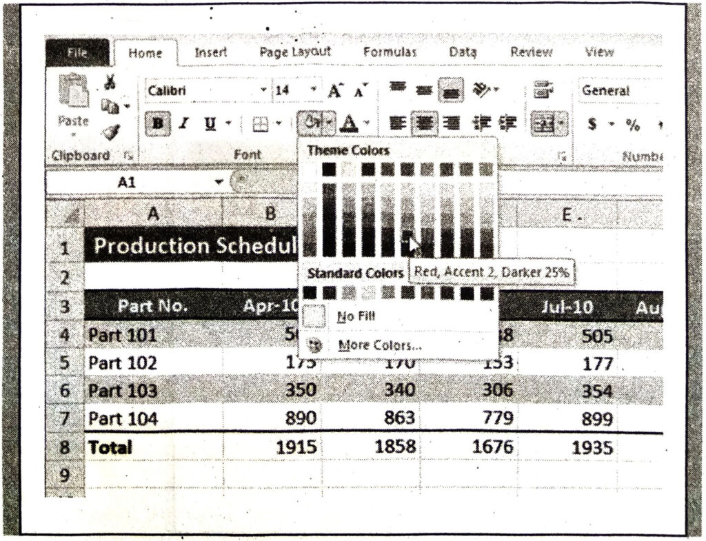
5. Basic Styles: There are some other styles available for text formatting. It includes:

(i) Bold, which makes our text a bit stronger than regular,

(ii) Italic, which is for making the text a little slanted,

(iii) Underline, which shows a line under the text to make them more emphasized.

Shortcut Keys:

(i) Bold — Ctrl + B

(ii) Italic — Ctrl + I

(iii) Underline — Ctrl + U

Changing the Cell Styles

There are several options for changing the styles of cells.

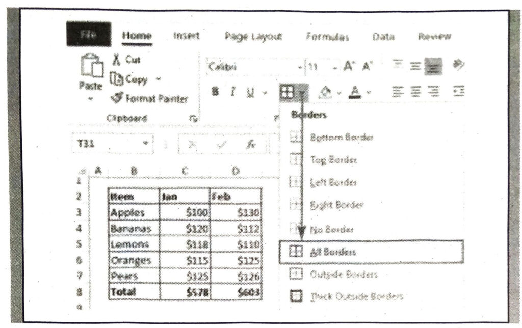
1. Cell Borders: Cell borders can be changed to have attractive presentation of data in spreadsheet. Border option can be used from Font group to apply border to a cell. Follow the steps:

(i) Select the required cells and press the arrow key of Border button. (A dropdown menu appears. It displays the different options for borders to apply.)

(ii) Select one or more option for a single selection.

More Borders option can be used to have advance setting of border using Format cell dialogue box.

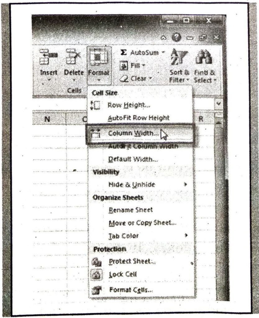
2. Changing Cell Width : The width of a cell can be changed by using this option. This width will be applied for entire column. Steps to change Cell Width are as follows:

(i) Select one or more columns.

(ii) Click on Format button in the Cells group of Home tab.

(A dropdown menu will appear. Choose column width option which will open Column Width Dialog Box.)

(iii) Enter the value of Column width.

(iv) Press OK button to apply cell width.

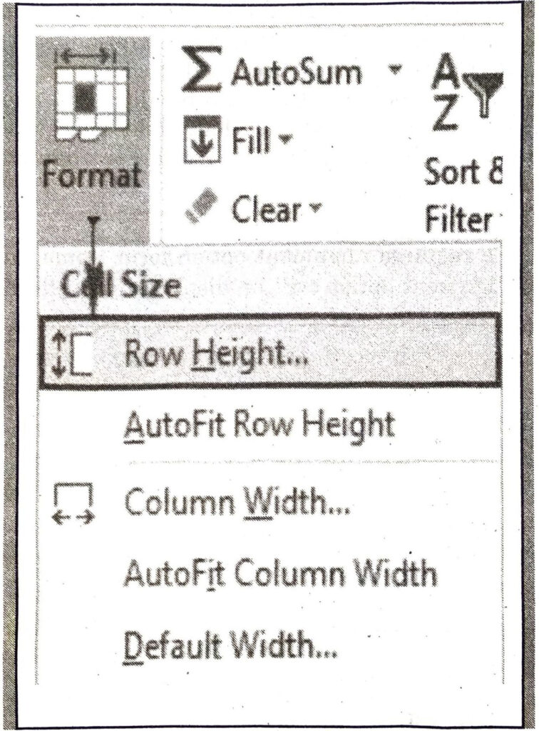
3. Changing Cell Height: The height of a cell can be changed using this option. This height will be applied for entire row. To change Cell height following steps are used :

(i) Select one or more rows.

(ii) Click on Format button in the Cells group of Home tab.

(A dropdown menu will appear. Choose Row Height option which will open Row Height Dialog Box.)

(iii) Enter the value of Row Height.

(iv) Press OK button to apply cell height.

4. Merging Cells: Merging the cells means to join two or more adjacent cells as a one. Any number of cells can be merged forming a rectangular area. If the cells being merged have contents, the information in the upper left cell will be retained. We can merge cells as follows:

(i) Select the cells to be merged.

(ii) Click on Merge and Centre from Alignment Group of Home tab ribbon.

(iii) Select further options of Merging from drop down menu appeared. The selected cells will get merged.

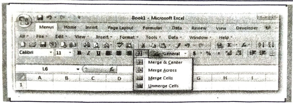
The Merge Across Option will merge each row of selected cells into a larger cell. Calls can be unmerged using “Unmerge” Option from the drop down.

5. Aligning Text: Contents of a cell can be aligned by using the Alignment group in the Home tab of ribbon. Contents can be aligned to the top, the bottom or the center. They can also be aligned left, right and center. Its just like the text in a word processing program like Word. For aligning the text, following steps are used :

(i) Select the Cells.

(ii) Choose the required alignment option form Home tab ribbon. The effect of each alignment option will be displayed on selected cells.

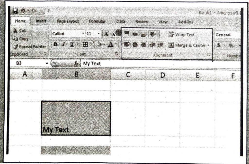
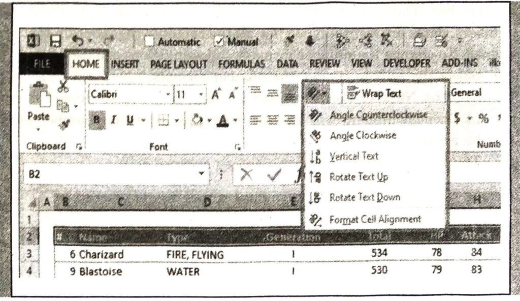
6. Changing Orientation of Text: Sometimes, column header is large than the data written under that particular field. In this case, change the orientation is required. Orientation of text can be changed within a cell as under :

(i) Select the cells whose orientation is to be changed.

(ii) Choose Orientation option of alignment group of Home Tab. (Different orientation options will be displayed in appeared drop down menu appeared.)

(iii) Select the required orientation.

Selected orientation will be displayed on selected cell.

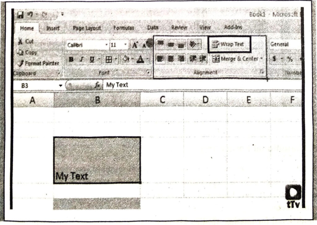
7. Wrapping Text: Sometimes contents go out of cell’s width. The text can be wrapped text within a same cell. For this purpose, Wrap Text option of Alignment Group in Home Tab Ribbon is used after selecting the particular cell or the range of cells.

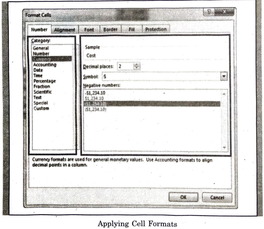
8. Applying Number Formats: The appearance of numbers in Excel can be changed without changing the values. The actual value is displayed in the formula bar. The default format for displaying numbers is General. All the numbers, dates are right aligned but all the contents that contain text are left aligned. To change the number formats, following steps are used :

(i) Select the cells to change the number formats.

(ii) Click on Number Format option of Number Group of Home tab ribbon.

(A Dropdown menu will appear. Select the particular number format to be applied.)

(iii) The Select Format will be applied on selected cells.

Conditional Formatting

Conditional Formatting is a tool in Excel that enables applying particular formats to a cell or range of cells depending on the value under specified condition. This tool is very useful. It can highlight the respective cells with certain formats to show valuable facts.

Conditional formatting applies one or more rules to any cell or range. Ahead steps are used to apply conditional formatting :

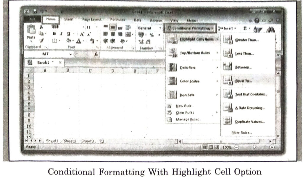
(i) Select the required cell or range where conditional formatting is to be applied.

(ii) Click on Conditional Formatting button from Home tab ribbon.

(Dropdown menu will appear and lot of pre-defined rules for conditional formatting will be displayed.)

(iii) Choose the required rule. Highlight cell rules can be used like Greater Than, Less Than, Between, Equal to, Duplicate Values etc.

(Dialog box related to selected rule will appear.)

(iv) Enter the values for the given rule.

(v) Press OK to apply specified Conditional Formatting.

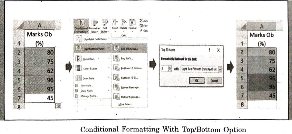
Some commonly used conditional formatting rules are Top/Bottom rules like Top 10 Items, Bottom 10 Items, Above average etc.

The steps for applying this type of rule will remain same.

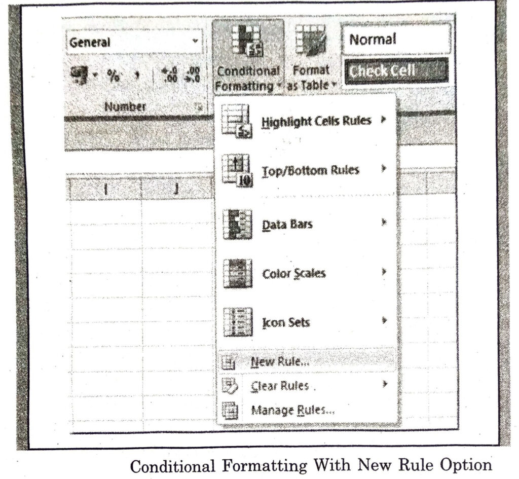
We can also create new rule for conditional Formatting using “New Rule” Option.

Formatting as Tables

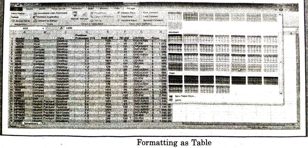
Excel, has several pre-defined formats. Formatting our spreadsheet can not only improve the look and feel of our spreadsheet. It also can make it easier to use. To apply this style of formatting, following steps are used :

(i) Select the cells to be applied formatting upon.

(ii) Click on Format as Table from Home tab.

(A new dialogue box will appear which shows a lot of different formats.)

(iii) Click the required format to be applied on the selected cells.

INSERTING ROWS, COLUMNS AND OTHER OBJECTS IN MS EXCEL

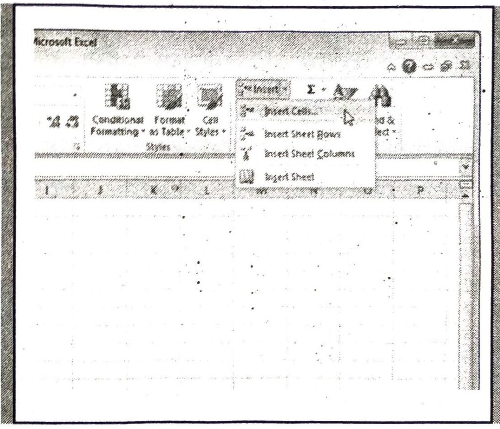
(i) To insert new cells, rows or columns in an Excel worksheet, Select the cellcells, rows, or columns where you want to insert a new cell or number of cells.

(ii) Click on Insert option of Cells group in Home Tab ribbon.

(iii) Select the desired option from the dropdown menu appeared.

Inserting Cells

(i) Select the cell where new Cell is to be inserted.

(ii) Select Insert Insert cell from Home tab ribbon.

(iii) Click on the required option and press OK.

Inserting Rows

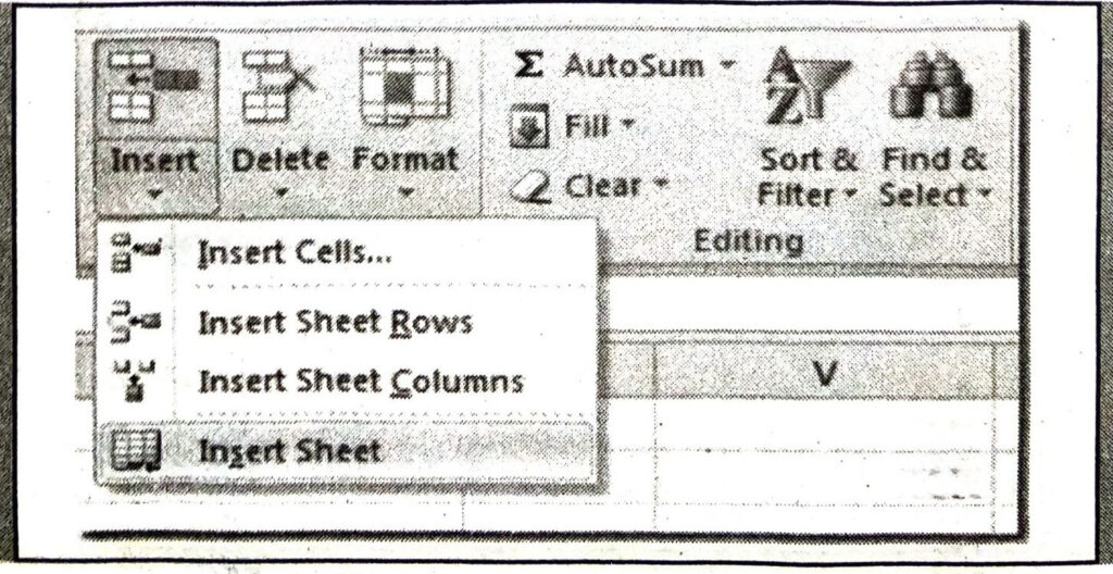
(i) Select the cell where new Row is to be inserted.

(ii) Select Insert Insert sheet rows from Home tab ribbon.

(iii) New row will be added on the place of selected cells.

Inserting Columns

(i) Select the cell where new column is to be inserted.

(ii) Select Insert -> “Insert sheet column” from Home tab ribbon.

(iii) New column will be added on the place of our selected cells.

Using Auto Sum

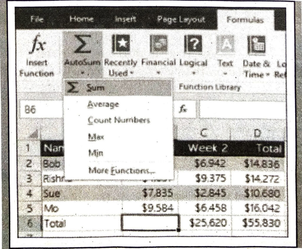
Functions in Excel are pre-defined formulas that are used to perform calculations. Excel provides a wide range of formulas like :

(i) sum (SUM),

(ii) average (AVERAGE),

(iii) count (COUNT, COUNTA),

(iv) maximum (MAX) and

(v) minimum (MIN).

Each of these functions is having its own specific operations to be performed. Any of these functions can be applied using “AutoSum” option from Editing group of Home Tab ribbon. Arrow key of AutoSum option can be used to use more functions.

Inserting Charts

Chart is a way to represent data graphically. Charts can be used for comparison, show relationship etc. Charts can be used for analysis also. Data should be entered in charts. What the data is changed, it is automatically reflected in charts.

Excel has various types of charts, so we can choose one that most effectively represents our data.

Types of Chart

1. Pie Chart 2. Column Chart 3. Line Chart 4. Bar Chart 5. Area Chart 6. Scatter Chart. 7. Surface Chart.

Create a Chart

To create a line chart, the steps are as follows:

(i) Type the data in our excel worksheet.

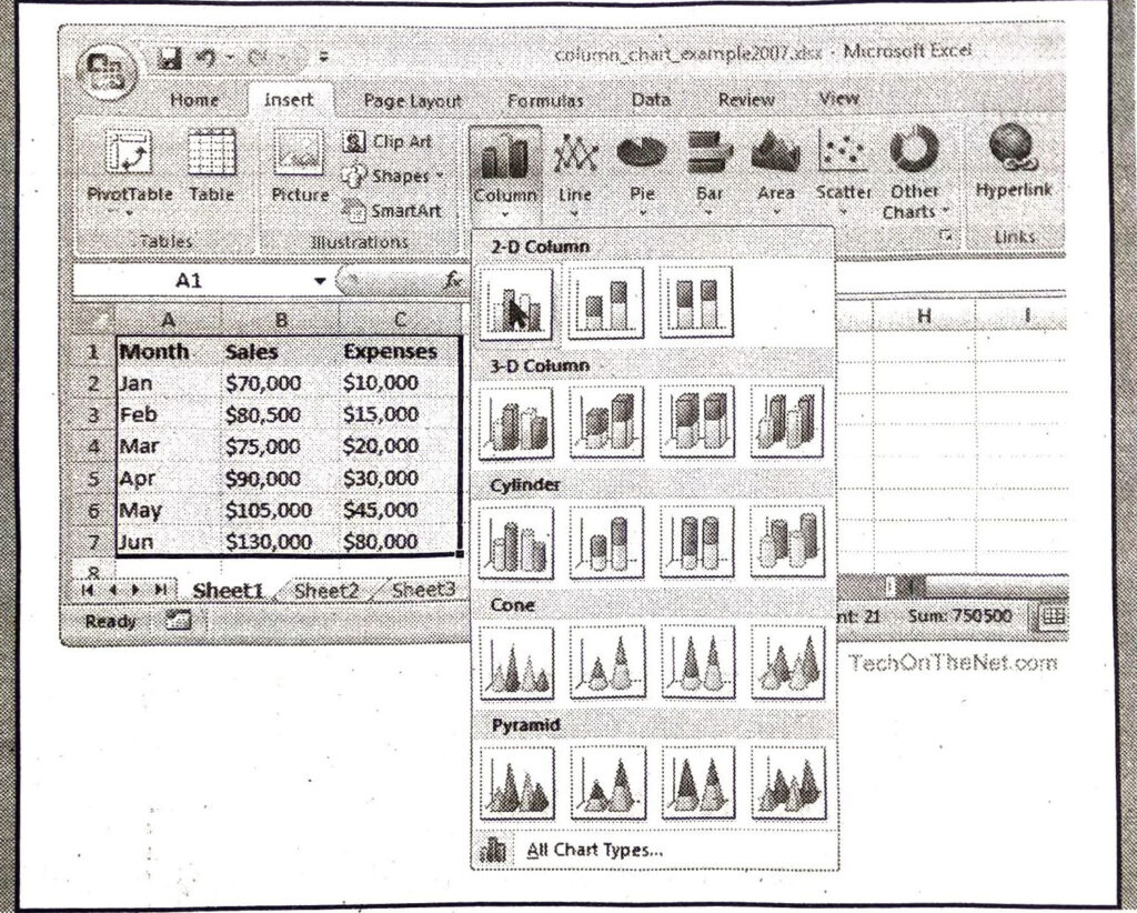
(ii) Click on layout tab → Chart Title → Above Chart

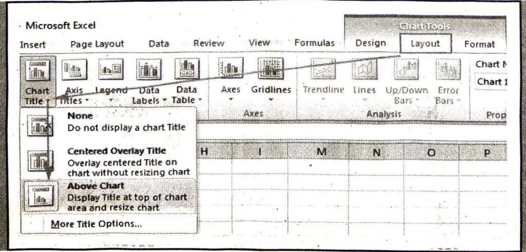
(iii) A caption will be displayed on chart. Type in the desired title.

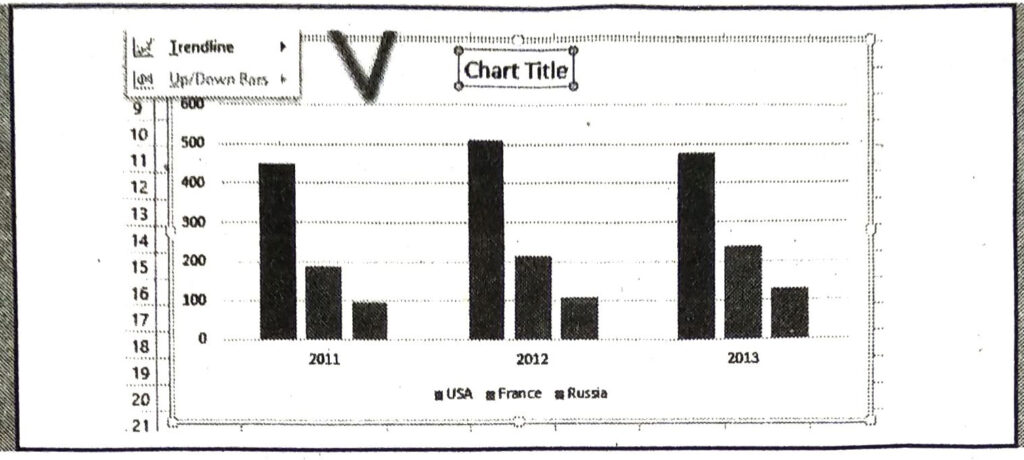
Add Chart Title

(i) Select the Chart.

(ii) On the Layout tab, click Chart Title, Above Chart.

(iii) We will see a caption (Chart Title) above our chart. Enter our desired title.

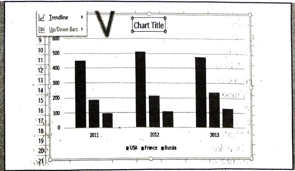
Elements of a Chart

1. Chart Area: A chart area contains everything inside the chart window, including all parts of the chart.

2. Data Marker: A data marker is a symbol on the chart that represents a single value in the worksheet. A data marker can be a bar in a bar chart, a pie in a pie chart or a line on a line chart.

3. Data Series: It is a group of related values such as all the values in a single Irow in the chart.

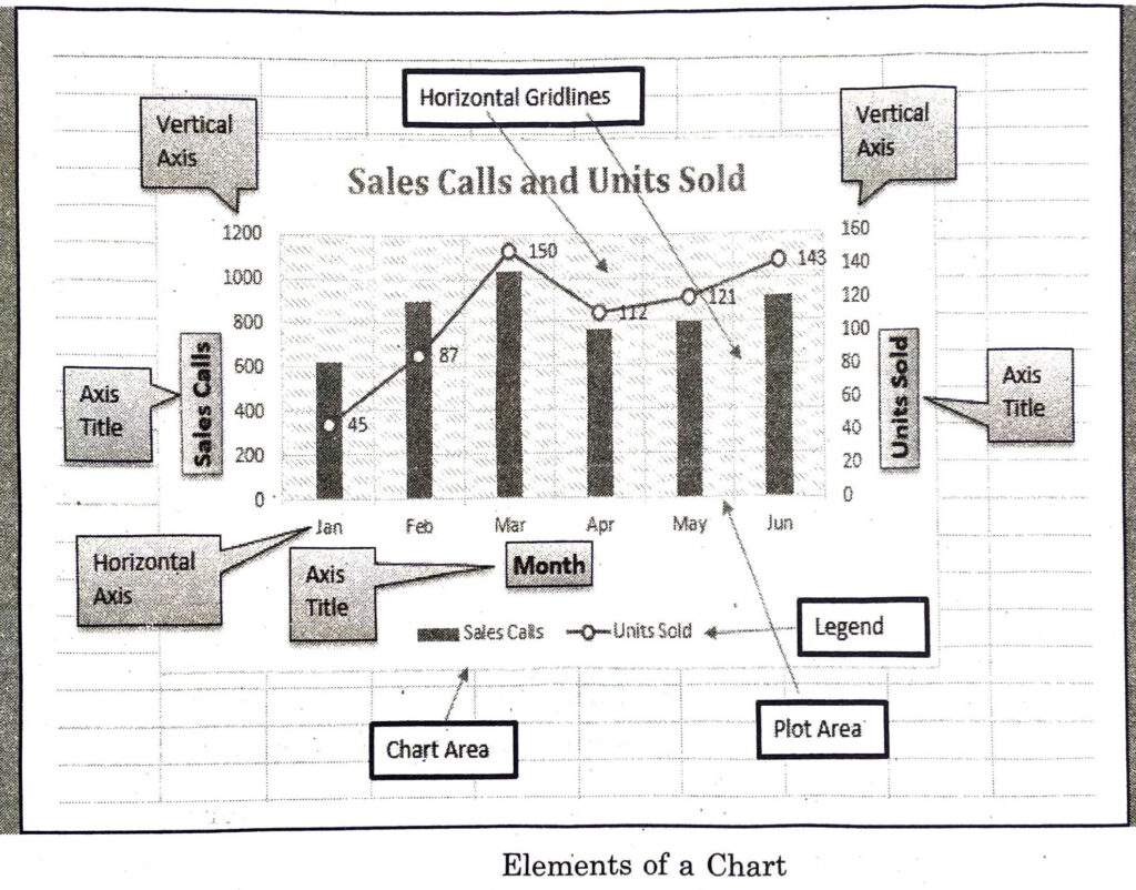
4. Axis: It is a line that is used as a major reference for plotting data in a chart.

5. Tick Mark: It is a small line intersecting an axis. A tick mark indicates a category, scale or chart data series.

6. Plot Area: It is the area where our data is plotted and it includes the axes and all markers that represent data points.

7. Gridlines: These are the optional lines extending from the tick marks across the plot area.

8. Chart Text: It is a label or title that we add to our chart. Attached text is a title or label that is linked to an axis such as the Chart Title.

9. Legend : It is a key that identifies patterns, colours or symbols associated with the markers of a chart data series. The legend shows the data series name corresponding to each data marker.

Computer Guide for Class 9 PSEB MS Excel Part-II Textbook Questions and Answers

Multiple Choice Questions :

1. By default, each new workbook in MS Excel 2010 contains ………. number of worksheets.

(A) 5

(B) 2

(D) 3.

Ans. (D) 3.

2. Which objects can be added in a worksheet?

(A) Cells

(B) Charts

(D) All of these.

Ans. (D) All of these.

3. Which are the valid types of Charts in MS Excel ?

(A) Bar, Column, Pie, Line

(B) Area, Doughnut, Scatter

(D) All of the above.

Ans. (D) All of the above.

4. Which function is used to find minimum number from the given range ?

(A) AVERAGE

(B) MIN

(D) RANK.

Ans. (B) MIN

5. ………………….. is a powerful tool of MS Excel used to have graphical representation of our data in MS Excel.

(A) Data Validation

(B) Conditional Formatting

(D) None of these.

Ans. (C) Charts

Write True or False :

1. New cell, row or column can be added by using Ctrl and + keys from keyboard.

Ans. True

2. SUM and MIN are examples of Chart Types in MS Excel.

Ans. False

3. Cell Borders, change cell width or height, Merge cells, Align Texts, Change Orientation of text, Wrap Text etc. are examples of cell styles.

Ans. False

4. Conditional Formatting is a tool in MS Excel that allows applying formats to a cell or range of cells depending on the value.

Ans. True

5. Formatting options effectively represents the information from facts of data.

Ans. True

Short Answer type Questions :

Q. 1. What do you mean by Formatting ?

Ans. Formatting is the process of changing the appearance of content in a file. it includes change of fonts, size of the fonts, background and foreground colour etc. the main purpose of formatting the text is to make it more beautiful and more readable.

Q. 2. Which type of formatting can be used as Cell Styles ?

Ans. Following type of formatting can be used as cell style

Changing the cell border
Changing the height and width of a cell
Merging cells,
Cell alignment

Q. 3. What do you mean by Merging Cells ?

Ans. Merging the cells means to join two or more adjacent cells as a one. Any number of cells can be merged forming a rectangular area. If the cells being merged have contents, the information in the upper left cell will be retained.

Q. 4. Define alignment and its types.

Ans. Alignment is the process of adjusting the text to a particular direction. Alignment can be of four types :

Left alignment
Right alignment
Centre alignment
Justified alignment

Q. 5. What are Charts ?

Ans. Charts are the graphical representation of data. it is an effective way to represent the data. the values of data are shown in various form in different types of charts. charts can be used for comparison showing relationship easily. they can also be used for data analysis.

Long Answer type Questions :

Q. 1. What is Conditional Formatting ? Explain its different options.

Ans. Conditional Formatting is a tool in Excel that enables applying particular formats to a cell or range of cells depending on the value under specified condition. This tool is very useful. It can highlight the respective cells with certain formats to show valuable facts.

Conditional formatting applies one or more rules to any cell or range. Following steps are used to apply conditional formatting :

(i) Select the required cell or range where conditional formatting is to be applied.

(ii) Click on Conditional Formatting button from Home tab ribbon.

(Dropdown menu will appear and lot of pre-defined rules for conditional formatting will be displayed.)

(iii) Choose the required rule. Highlight cell rules can be used like Greater Than, Less Than, Between, Equal to, Duplicate Values etc. Dialog box related to selected rule will appear.

(iv) Enter the values for the given rule.

(v) Press OK to apply specified Conditional Formatting.

Some commonly used conditional formatting rules are Top/Bottom rules like Top 10 Items, Bottom 10 Items, Above average etc.

Q. 2. What are charts ? Give the name of any five types of charts.

Ans. Chart is a way to represent data graphically. Charts can be used for comparison, show relationship etc. Charts can be used for analysis also. Data should be entered in charts. What the data is changed, it is automatically reflected in charts.

Excel has various types of charts, so we can choose one that most effectively represents our data.

Types of Chart

(i) Pie Chart.

(ii) Column Chart

(iii) Line Chart

(iv) Bar Chart

(v) Area Chart

(vi) Scatter Chart

(vii) Surface Chart.

Q. 3. Explain any three objects which can be added in MS Excel worksheet.

Ans. The process of adding three object i.e. cells, rows and charts are as given below :

1. Inserting Cells:

(i) Select the cell where new Cell is to be inserted.

(ii) Select Insert Insert cell from Home tab ribbon.

(iii) Click on the required option and press OK.

2. Inserting Rows:

(i) Select the cell where new Row is to be inserted.

(ii) Select Insert Insert sheet rows from Home tab ribbon.

(iii) New row will be added on the place of selected cells.

3. Inserting Charts:

(i) Type the data in our excel worksheet.

(ii) Select the range.

(iii) On the Insert tab, in the charts group, choose line and select line with markers.

PSEB 9th Class Computer Guide MS Excel Part-II Important Questions and Answers

Fill in the Blanks :

1. An Excel workbook contains ……………….. .

(A) Worksheets

(B) Rows

(D) Formula

Ans. (A) Worksheets

2. The value or content of a cell is displayed in ……………….. .

(A) Title

(B) Menu

(D) none of the above

Ans. (C) Formula bar

3. Using ………… type of formatting we can change the cell style by applying more than one rules.

(A) Formula

(B) Function

(D) none of the above

Ans. (C) Conditional

4. Format command is available on ………….. menu.

(A) Home

(B) Insert

(D) Formula

Ans. (A) Home

5. All the formulas start with the sign ……………………. .

(A) Sigma

(B) Addition

(D) None of the above

Ans. (C) Equal to

6. Data in a worksheet can be arranged in a special order using …………….. command.

(A) Formula

(B) Function

(D) Sorting

Ans. (D) Sorting

7. Sort and filter command are available ……………. tab.

(A) Home

(B) insert

(D) None of the above

Ans. (C) Data

8. Format cell window contain ……………. tabs.

(A) 5

(B) 6

(D) 8

Ans. (B) 6

9. Excel contains ……………… number formats.

(A) 6

(B) 8

(D) 12

Ans. (D) 12

10. ……………. options are available in insert/ delete dial.

(A) 4

(B) 5

(D) 7

Ans. (A) 4

11. Workbook contains ……………… worksheet at the starting.

(A) 2

(B) 3

(D) 5

Ans. (B) 3

12. …………… contains everything inside the chart window.

(A) Data markers

(B) Axis

(D) None of these.

Ans. (C) Chart area

13. …………….. feature allows you to set up certain rules.

(A) Data validation

(B) Pivot Table

(D) None of these.

Ans. (A) Data validation

14. We can ……………… the worksheet window into separate panes.

(A) Hide

(B) Split

(D) None of these.

Ans. (B) Split

15. By using ……………… you can keep rows or columns visible while scrolling.

(A) Hide

(B) Split

(D) None of these.

Ans. (C) Freeze Panes

Write True/False :

1. We cannot change the font colour in Excel.

Ans. False

2. Two cells can be merged to make one cell in Excel.

Ans. True

3. New rows can be inserted in Excel worksheet.

Ans. True

4. Graphical representation of data is called table.

Ans. False

5. Column cannot be inserted in Excel.

Ans. False

Short Answer Type Questions :

Q. 1. What is a cell style ?

Ans. Cell styles are the predefined formatting options which are available in excel and are used to format a cell.

Q. 2. Write the name of different types of charts available in Excel.

Ans. Different Types of charts available in excel are :

(i) Pie chart

(ii) Column chart

(iii) Line chart

(iv) Bar chart

(v) Area chart

(vi) Sector chart.

Q. 3. Write the name of any five elements of a chart.

Ans. The names of elements of are:

(i) Title

(ii) Axis

(iii) Chat area

(iv) Data series

(v) Legend

Q. 4. What do you mean by chart ?

Ans. Chart is a graphical representation of data. Data can be shown in different formats using charts.

Q. 5. Explain the basic text styles in style in Excel.

Ans. Excel contains some basic Textiles which can be used on the content of a cell. Styles are:

(i) Bold

(ii) Italic.

(iii) Underline

Q. 6. What do you mean by merging cells ?

Ans. The process of combining two or more cells to make one cell is called merging of cells. In this process the content of the first cell remains in the final merged cells. Cells can be merged across rows or columns.

WNA24

PSEB Solutions for Class 9 Computer Science Chapter 4 MS Excel Part-II

PSEB 9th Class Computer Solutions Chapter 4 MS Excel Part-II

INTRODUCTION

Computer Guide for Class 9 PSEB MS Excel Part-II Textbook Questions and Answers

Leave a Reply Cancel reply