PSEB Solutions for Class 9 Computer Science Chapter 5 MS Excel Part-III
PSEB 9th Class Computer Solutions Chapter 5 MS Excel Part-III
INTRODUCTION OF FORMULAS AND FUNCTIONS
A formula is an expression that operates on values in a given range of cells. Many operators can be used within a formula. They describe the required operation to-be performed on data.
A function is a predefined formula that performs calculations upon specific values in a particular order. Excel spreadsheet program includes common functions like Sum, Average, Count, If, SumIf, CountIf, Max, Min, etc. and many more.
Steps to use function in Excel: Following steps are used to use a function in Excel :
- Select the cell in which function is to be used
- Type in the equal to sign
- Type the name of the function
- Write the arguments in the bracket after the name of function
- Press the enter key
Difference between Function and Formula
Differences between function and formula are :
| Function |
Formula |
| 1. Function is pre defined in Excel. |
1. Formula is created by the user. |
| 2. Function has a particular name. |
2. Formula does not have a name. |
| 3. Function can be used by typing or by selecting. |
3. Formula is used by typing only. |
| 4. Mathematical signs and symbols are hidden in a function. |
4. Mathematical signs and symbols visible in a formula. |
| 5. Function is easy to use. |
5. Formula is difficult to use. |
Elements of Formulas
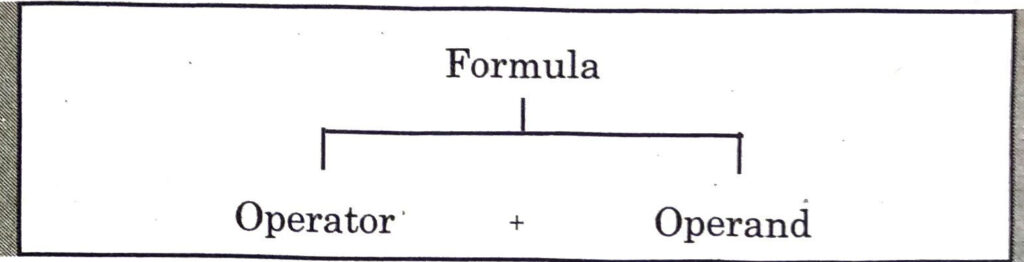
A formula is an expression. It is used for calculation. These expressions are userdefined. These can be as small as well as complex enough to perform some advanced calculations. These expressions can be designed using constant values, cell references and operators. Each expression can have two parts:
- Operators: Operator defines what to do on the data. Various symbols representing different operation known as “operators” for defining operation of expression are used for this purpose.
- Operands: Operand defines the values on which the given operation is to be applied. Each operator have particular operand requirement. Some operators require one operand and some require two or more operands.
Operators used in MS Excel Formulas
Operators are the symbols which represent a particular operation to be performed. Excel follows mathematical rules on operators for calculations. The precedence of operators in an expression would be Parentheses, Exponents, Multiplication and Division, Addition and Subtraction etc. The four types of calculations used in Excel are arithmetic, comparison, text concatenation and reference.
1. Arithmetic Operators: These operators are used to perform arithmetic operations. These operators are :
Arithmetic Operators
| Symbol |
Arithmetic Operator |
Meaning |
Example |
Result |
| + |
plus sign |
Addition |
= 3+3 |
6 |
|
–
|
minus sign
|
Subtraction
Negation
|
= 3-3
= -3-3
|
0
-6
|
| * |
asterisk |
Multiplication |
= 3*3 |
9 |
| / |
forward slash |
Division |
=3/3 |
1 |
| % |
percent sign |
Percent |
= 30% |
0.3 |
| ^ |
caret |
Exponentiation |
= 3^3 |
27 |
2. Comparison Operators: These operators are used for comparison. Only logical values are given as a result after using these operators i.e. either TRUE or FALSE.
Comparison Operators
| Symbol |
Comparison Operator |
Meaning |
Example |
| = |
equal sign |
Equal to |
=A1=B1 |
| > |
greater than sign |
Greater than |
=A1>B1 |
| < |
less than sign |
Less than |
=A1<B1 |
| >= |
greater than or equal to sign |
Greater than or equal to |
=A1>=B1 |
| <= |
less than or equal to sign |
Less than or equal to |
=A1<=B1 |
| <> |
not equal to sign |
Not equal to |
=1<>B1 |
3. String Concatenation Operator: Strings are also known as text contents. Ampersand (&) is usèd to concatenate (join) one or more text strings as a single text.
Table String Concatenation Operator
| Symbol |
Text operator |
Meaning |
Example |
Result |
| & |
Ampersand |
Connects or concatenates, two values to produce one continuous text value |
=”North” & “wind” |
Northwind |
The Operators Precedence in Excel
Operator Precedence
| Sr No. |
Operator |
| 1 |
Exponentiation (^) |
| 2 |
Multiplication (*), Division (/) |
| 3 |
Addition (+), Subtraction (-) |
| 4 |
Concatenation (&) |
| 5 |
All Comparison Operators
|
Cell Referencing
Cell reference is a way to name address of a particular cell, group of cells or a range. The way of representing the cell addresses within a formula or function is called Cell Referencing. When a cell reference written in a cell as a part of any function or formula is copied to another cell then the references given in the cell changed accordingly. This feature is very useful for application of formulas over multiple cells without making changes. Sometimes references are required to be constant after being copied. For this, options are also given in Excel.
The different types of cell referencing are :
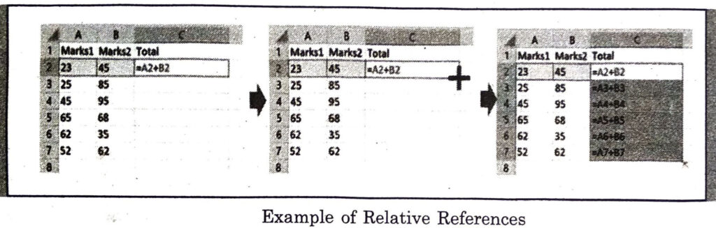
1. Relative References: When relative referencing is copied to another location, it changes based on the relative position of rows and columns. This is a default referencing in MS Excel. For example, if we copy the formula = A1 + B1 from row 1 to row 2, the formula will become = A2 + B2.
Relative references are especially convenient when same calculation is repeated over multiple rows or columns.
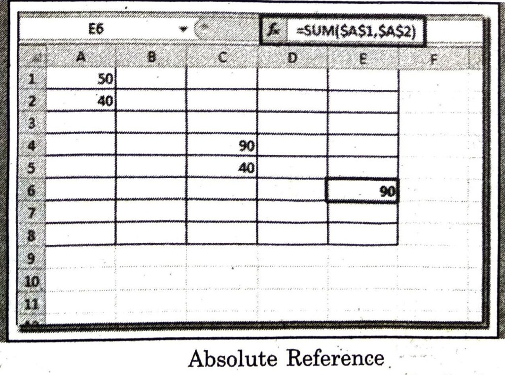
2. Absolute Reference: Absolute references do not change when copied or filled. Absolute reference can be used to keep a row or column constant. An absolute reference is designated in a formula by the addition of a dollar sign ($) before column and row.
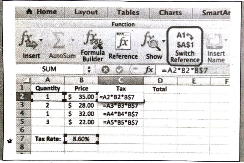
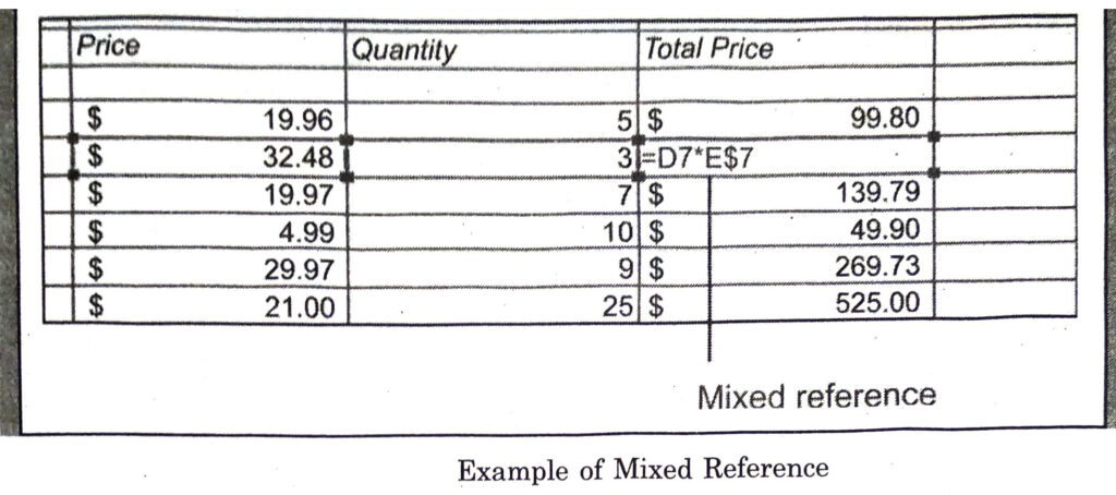
3. Mixed Reference: This referencing is a mixture of both absolute and relative reference. Only one out of a row or a column remain fixed while copying. This type of reference is used in special kind of situations.
USES OF FORMULAS AND FUNCTIONS
The use of formulas and functions can be seen from following discussion :
Using Formulas
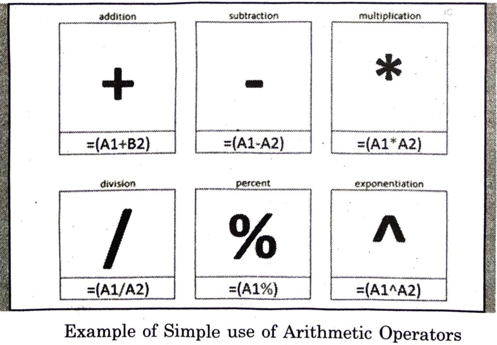
1. Simple use of Arithmetic Operators: This is a simplest type of formula which performs basic calculations. This type of formula is having different arithmetic operators applied on one or two values.
Explanation :
Explanation of Simple use of Arithmetic Operators
| S.No. |
Formula |
Description |
| 1 |
= A2 + B2 |
Only one operation with two cell reference. |
| 2 |
= A3 + B3 + C3 |
Only one operation with more than two cell reference. |
| 3 |
= A4 + B4 – C4 |
Multiple operations with more than two cell reference. |
| 4 |
= A5 + 10 + C5 |
Only one operation with cell reference and constant values. |
| 5 |
= A6 + B6 – C6 + 3 |
Multiple operations with cell reference and constant values. |
2. Advanced Use of Arithmetic Operators with Operator Precedence : Advanced formulas with more than one operator can be developed within a single expression. One has to take care of operator precedence. It is the order of execution of operators when multiple types of operators are used within a same statement.
Explanation:
Explanation of Advanced Use of Arithmetic Operators
| S.No. |
Formula |
Description |
| 1 |
= (A2 * 10) + 2 |
Two operators are used. * is having highest precedence so the result will remain same with and without parentheses. |
| 2 |
= (A3 + B3) * 10 |
Here operator is put in parentheses which is having lower precedence over *. Here the result will be changed if parenthesis are not used. |
| 3 |
= A4 * 2 + B4 * 5 |
Description If two operators with equal precedence are put in single formula then both these would be executed at a same time. So, here + will be executed after execution of both * operators. |
| 4 |
= A5 * B5 + A5 |
Here again will be executed prior to + operator. |
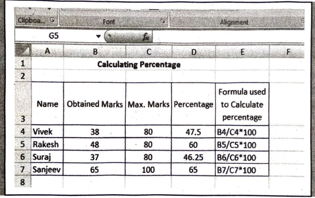
3. Using Formula for calculating the Percentage: Calculating percentage is one of the most common tasks to be used in any of the application.
We can apply this formula in MS Excel data of student marks as follows:
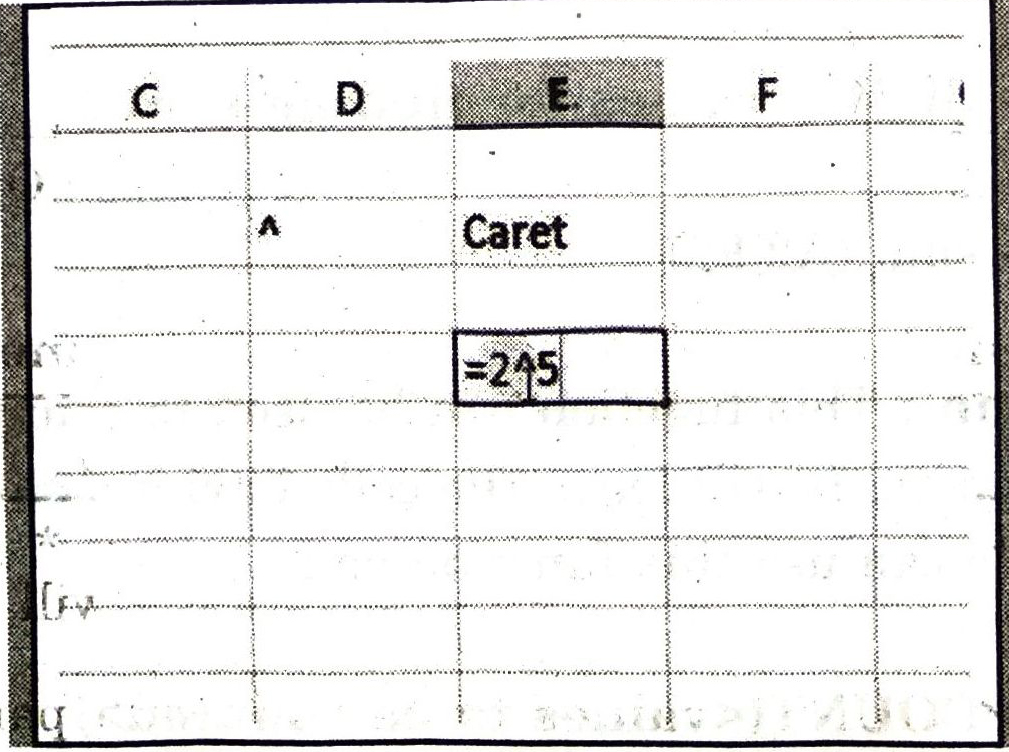
4. Using Caret (^) Operator: This operator is used to find the power of any given value. This operator is applied between two operands. Such as, if this operator is applied as = A^ B, then it will calculate AB.
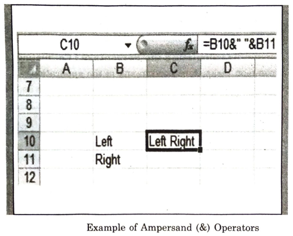
5. Using Ampersand (&) Operator: This operator is used to join two string values. This operator can be applied on text data values only. More than one ampersand (&) operators can be used within a single statement. This is an alternate of CONCATENATE function of Excel.
Using Functions
Excel includes many functions that can be used to perform required calculations on given a range of cells. Functions can be categorised in several categories..
1. Mathematical Function
These functions are mainly used for mathematical calculations. Such as:
(1). SUM Function: This function is mainly used for finding the sum of values provided in given cells or range. We can use this function as :
Syntax:
= SUM (<values for finding sum>)
Example :
= sum (A2:F2)
(2). COUNT Function: This function can be used to count the number of cells that contain numbers. It will leave the cells having non-numeric values from being counted. We can use this function as :
Syntax :
= COUNT(<values to be counted>)
Example :
= count (A2:F2)
(3). COUNTA Function: This function is used to count all the cells having any type of contents. Only those cells will be left from counting in a range that are empty.
Syntax :
= COUNTA (<values to be counted>)
Example :
= counta (A2:F2)
(4). COUNTBLANK Function: This function is used to count only the blank cells in a range selected.
Syntax :
= COUNTBLANK (<values to be counted>)
Example :
= countblank (A2:F2)
(5). AVERAGE Function: This function is used when we want to get the average (arithmetic mean) of the specified group of cells or range.
Syntax :
= AVERAGE (<values to find average>)
Example:
= Average (A2:F2)
(6). MIN Function: This function is used when we want to find the minimum number from a group of cells or range selected as a result.
Syntax :
= MIN(<values, out of which minimum no is to find>)
Example :
= Min (A2:F2)
(7). MAX Function: This function is used when we want to find the maximum number from a group of cells or range selected as a result.
Syntax :
= MAX(<values, out of which maximum no. is to find>)
Example :
= Min(A2:F2)
(8). RANK Function: This function provides the rank to the selected cell or value within a selected range.
Syntax :
= RANK (<group of all values>, <value whose rank is to find>)
Example:
= rank(A2:F2, A2)
(9). LARGE Function: This function gives the Nth largest number from a group of cells or range.
Syntax :
= LARGE (<group of all values>, <value of N to find th largest no>)
Example:
= Large (A2:F2, A2)
(10). ROUND Function: This function is used to round a number to the given number of digits. If we give number of digits in negative then it will round the number before decimal point with 10s.
Syntax :
= ROUND (<value>,<significance of round off>)
Example:
= Round (A2,2)
2. Conditional Functions
These functions are used to perform calculation based on some condition. Some of the conditional functions are as under :
(1). IF Function: This function is used to perform some particular operation based operator on a comparison . It’s main function is decision making.
Use of IF Function: IF function can be applied simply by giving one comparison operator and based on that operator, two different operations or values can be given.
Syntax :
= If (Condition, ‘Result 1’, ‘Result 2’)
Example :
= If (A2<40, ‘Fail’, ‘Pass’)
Complex conditions used in IF Function: IF function can also be used for any complex operation. One if can be used in another if. This is also called nested if.
(2). SUMIF Function: Sum of any specific value can be found from the given range or group of cells by using this function.
Syntax :
= SUMIF (<group of values>, <value as a criteria>)
Example :
= Sumit (A2: A12, 8)
(3). COUNTIF Function: Number of cells having any specific value from the given range or group of cells can be found using this function.
Syntax:
= Countif (< group of values >, value is a criteria >)
Example:
= Countif (A2: A12, 8)
3. String Functions
String functions are used on text data. Many different operations can be performed using these functions on text data.
(1). LEN Function: This function is also called Length function. Number of characters including spaces and symbols within a string can be found using this function.
Syntax:
= LEN (< string value >)
Example:
= Len (A2)
(2). LEFT Function: Left part of string for any length provided by the user can be found with the help of this function.
Syntax:
= LEFT (< string value > < length in numbers >)
Example :
= Left (A2, 8)
(3). RIGHT Function: Right part of string for any length provided by the user can be found with the help of this function.
Syntax :
= RIGHT (< string value > < length in numbers >)
Example :
= Right (A2, 8)
(4). MID Function: This function is used to find the specific character from the middle of string to the specific number of characters of a string.
Syntax :
=MID (<string value>, <string position >, <required length>)
Example :
= Mid (A2, 4, 5)
(5). LOWER Function: This function is used to convert the characters of whole string to the lower case.
Syntax:
= LOWER (< string value >)
Example :
= Lower (A2)
(6). UPPER Function: This function is used to convert the characters of whole string to uppercase.
Syntax:
= UPPER (< string value >)
Example:
= Upper (A2)
(7). PROPER Function: This function is used to change the case of whole string in such a way that the first letter of each word would become CAPITAL and all rest of the letters will become small after using this function.
Syntax :
= PROPER (< string value >)
Example :
= Proper (A2)
(8). TRIM Function: Trim Function is used to delete the extra space from the string from both ends. This function will not delete the single space between the words and will delete all the extra leading and trailing spaces in the string.
Syntax :
= TRIM (string value)
Example:
= Trim (A2)
4. Date Functions
These functions are used to manipulate dates in Excel. There are several date functions for different purposes.
(1). TODAY Function: This date function returns the system date as a result. The format of date depends upon the system setting for Date and Time option.
Syntax :
= TODAY ( )
(2). NOW Function: This function returns the date of a system in conjunction with the current time. This time will be updated automatically when the sheet is opened or the formula is refreshed by editing it.
Syntax :
= NOW ( )
(3). DAY Function: This function returns day part of the date given as an argument.
Syntax :
= DAY (<date value>)
(4). MONTH Function: This function returns Month part of the date given as an argument.
Syntax :
= MONTH (<date value>)
(5). YEAR Function: This function returns Year part of the date given as an argument.
Syntax :
= YEAR (<date value>)
SORTING AND FILTERING DATA
Sorting and Filter are very useful options of Excel.
Sorting Data
Sorting data means to rearrange the rows based on the contents of a particular column in particular order. The process of sorting data in Excel can be applied different ways.
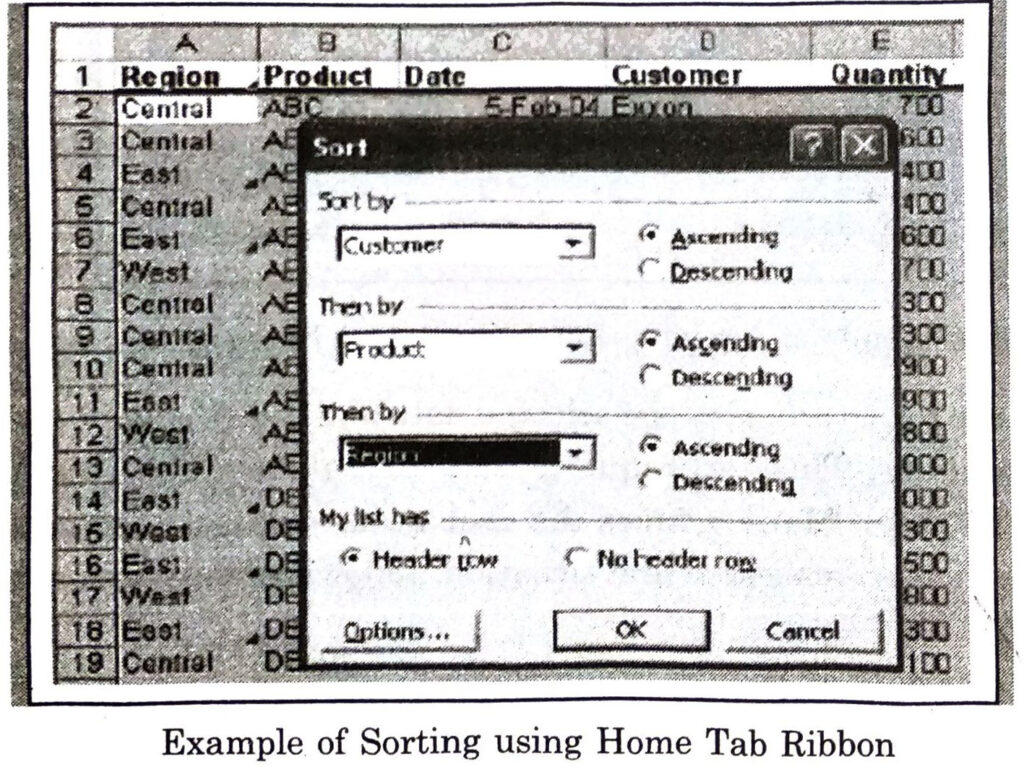
Sorting using Home tab ribbon
This is a simplest form of sorting data in Excel. In this method, the selected data is sorted in the particular order using last column of the selection. Multiple columns can not be used in this method of sorting. To apply sorting following steps are used :
- Select the required data to be sorted.
- Click “Sort & Filter” button from Home tab ribbon.
- Select the sorting order from the Dropdown menu appeared. Our selected data would be get sorted.
Sorting Data using Data Tab
Sort Option of Data Tab ribbon is used to sort the data on any other column of the data. The steps are as follows:
- Select Sort option from Data Tab.
- Select the columns to sort
- After this process, when OK button is pressed, the selected data is sorted according to column given in an ascending manner.
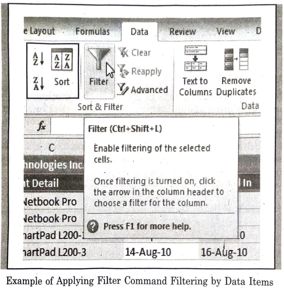
Filtering Data
Filter option is used to show data after hiding particular parts of unwanted data. ahead given steps are used :
- Prepare our data as per the availability of different options.
- Select the data to be filtered.
- Select “Filter option”from Data Tab Ribbon.
- Filter Option will be applied as shown below :
In Excel filters are used to display the selected data and hide the undesired data from the user or analysis. This technique is very useful for analysing the data for manipulating the data. Many a times the user needs only selected data from large amount of data. Filters are used in that situation. following steps are used for filtering the data.
(i) Create your data as per your requirement.
(ii) Select the data you want to filter.
(iii) Select data from filter tab.
(iv) Select the criteria to filter the data.
(v) The data will be filtered.
- Filtering by data items: After selecting the filter command small Arrow is displayed on each column of the collected data. Filter can be applied from the small arrows as per our requirement and selecting the criteria for filtering the data.
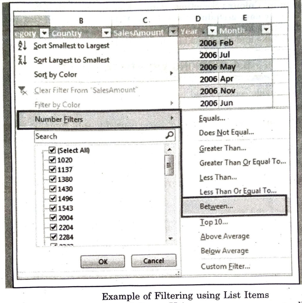
- Filtering the data according to range of data : This option is used to select the data which lies within a particular range of data. This option is mainly used on America data. Ahead given steps are used to filter the data in using this option.
Filtering according to range of data : Using this option of filter, all the rows as a result of filter which are having data value in a particular range of data are filtered. A new dialog box “Custom Auto Filter” appeared. Required filter can be created as one or two conditions with different options and using “and”, “or” operators between those operators.
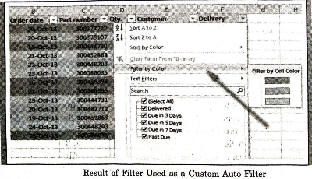
3. Filtering by Colour: Sometime, data is highlighted with different colours. It is needed to filter data according the colours. Both fill color and text color can be used for this option. Filter by choosing “Filter by colour” option from filter menu can be used in this case and then clicking the particular colour.
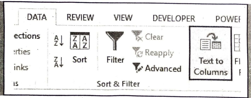
WORKING WITH DATA TOOLS
Excel also provide some special tools. These tools are used for special purposes. Few of these are :
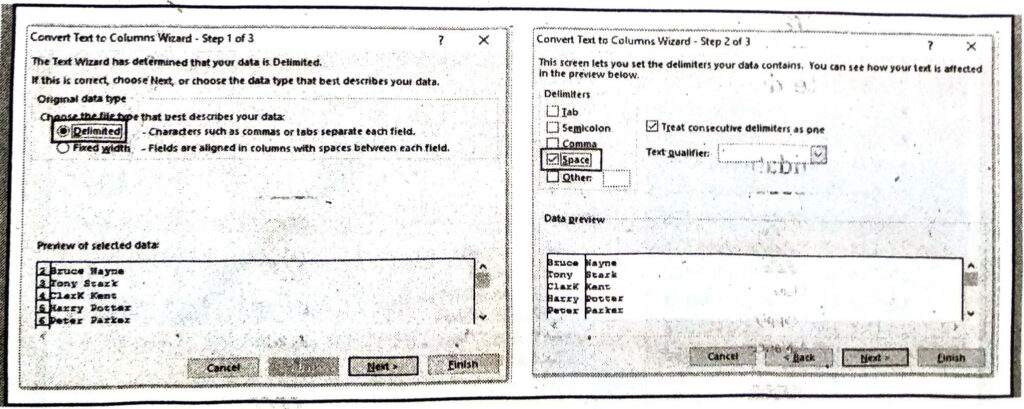
1. Text to columns : This option of Excel is used to split contents according to a fixed length or any particular symbol (like comma or space or any other) into different cells. This option can be applied by using “Text to Columns” option from Data Tab Ribbon after selecting the cell having contents to be split. The steps to use this feature are :
(i) Type the data in worksheet.
(ii) Select the range.
(ii) Clik Text to Columns on data Lab.
(A Dialog box will appear)
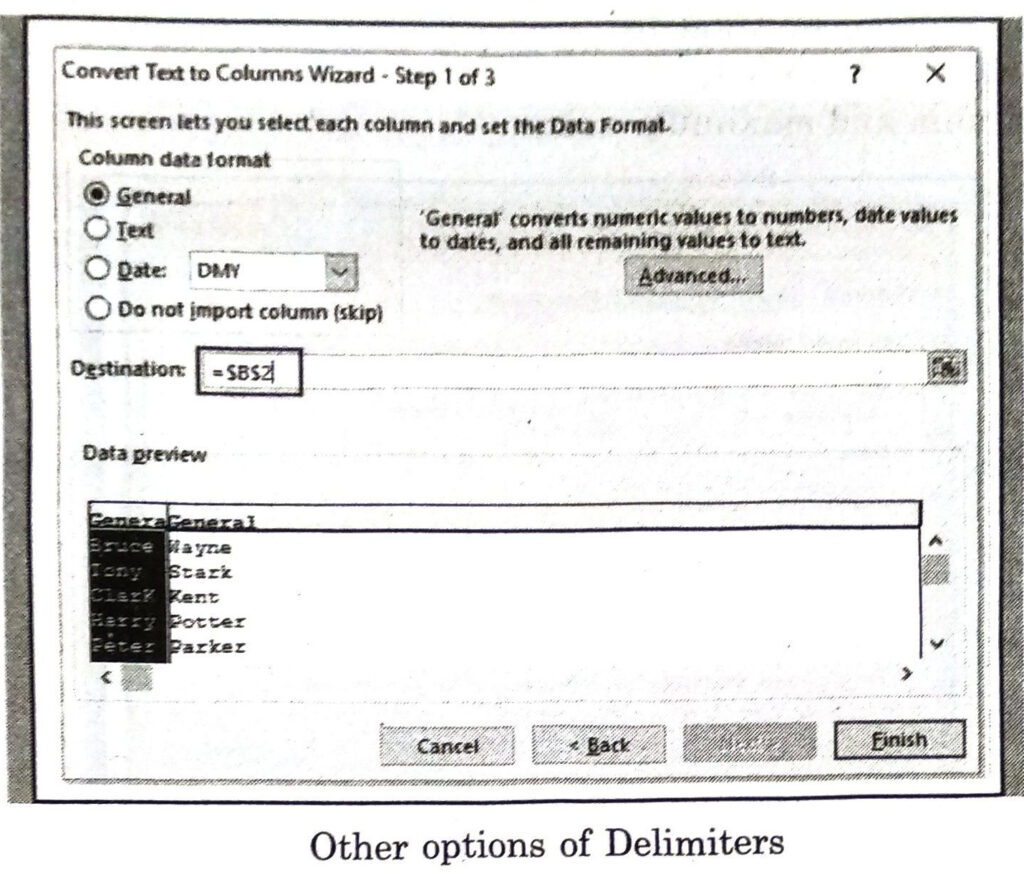
(iv) Select the delimited and click next.
(v) Clear all the check boxes
(vi) Click on Finish.
2. Remove Duplicates : This option of Excel can be very useful when there is dulicate data. This can be used from Data Tab Ribbon. “Remove Duplicates” option from Data tab ribbon is used after selecting the cells..
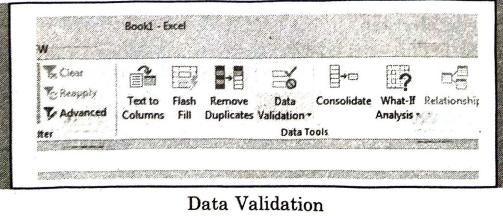
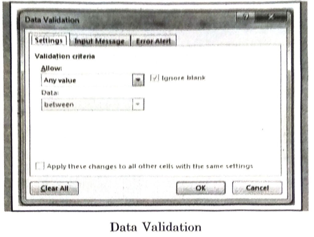
DATA VALIDATION
This option is very useful in those cases where we have any column in which only some particular values are allowed to be entered. If the value entered does not meet the given criteria, a specific error message is displayed. Several options are available in Excel. This tool can be used by selecting Data Validation option from Data Tab Ribbon after selecting the required column or cells.
To Create Data Validation Rule
The steps to create data validation are:
(i) Select the cel;.
(ii) Select Data Validation from Data Tab.
Do as directed on setting tab
(iii) Click whole number in Allow list.
(iv) Click Between on Data list.
(v) Enter minimum and maximum value.
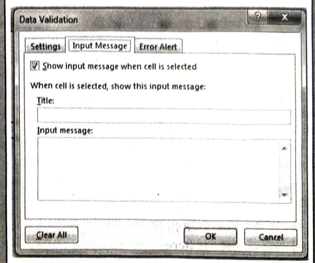
Input message :
Input message is displayed when the user select the cell on which data validation is applied. This on input message tab:
(i) Select the option Show input message when cell is selected.
(ii) Enter appropriate title.
(iii) Enter input message.
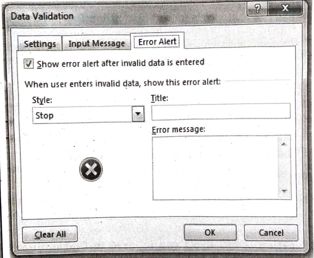
Error Alert:
If a user ignores the input message and enter wrong data then error alert is displayed. Following steps are used to set error alert.
(i) Click on error alert tab.
(A dialog box will be displayed)
(ii) Select option Show error alert when invalid data is entered.
(iii) Enter the Litle.
(iv) Enter the error alert.
(v) Click on OK.
Computer Guide for Class 9 PSEB MS Excel Part-III Textbook Questions and Answers
Fill in the Blanks :
1. Each function or formula must start with ………………. symbol in MS Excel.
(A) +
(B) =
(C) &
(D) ^
Ans. (B) =
2. Which function of MS Excel can be used to find minimum numbers from given range ?
(A) Minimum
(B) Mid
(C) Min
(D) None of these.
Ans. (C) Min
3. Ampersand (&) symbol is an alternate of …………….. function in MS Excel.
(A) Sum
(B) And
(C) Concatenate
(D) Power.
Ans. (C) Concatenate
4. Which data tool can be used to have only distinct values in a particular column ?
(A) Data Validation
(B) Text to Columns
(C) Formula
(D) Remove Duplicates.
Ans. (D) Remove Duplicates.
5. Which one is an example of Arithmetic Operator?
(A) +
(B) %
(C) ^
(D) All of these.
Ans. (D) All of these.
Write True or False :
1. We cannot count blank cells in MS Excel.
Ans. False
2. Formula is an expression of operators and operands to perform calculations.
Ans. True
3. SUM function can be used to perform addition of values in a particular range.
Ans. True
4. Text to columns option can be used to split our contents in multiple cells.
Ans. True
5. NOW function returns current data and time in MS Excel.
Ans. True
Short Answer Type Questions :
Q. 1. Write arithmetic operators being used in MS Excel.
Ans. Arithmetical operator are used to perform Arithmetic operations on given data. There are many arithmetical operator used in Excel. These operators are similar to the operators used in Arithmetic. These operators are the addition(+), subtraction (-), multiplication(*), division(/), percentage (%) and exponent (^).
Q. 2. What do you mean by Data validation ?
Ans. Data validation is a process to restrict the wrong input of data to various cells. Certain rules are formed for entering the data in those cells. Excel calculate the entered data as per the rules formulated. If the invalid data is entered in the cell then an error message is displayed.
Q. 3. Give the name of any three mathematical functions.
Ans. The names of three mathematical functions are :
(i) Sum
(ii) Average
(iii) Count.
Q. 4. What is sorting in MS Excel ?
Ans. Sorting data means to rearrange the rows based on the contents of a particular column in particular order. The process of sorting data in Excel can be applied in different ways.
Q. 5. Define formula.
Ans. Formula is an expression which is framed by the user to calculate. It uses values for the content entered in the various shelf for calculation. If formula in itself is a special combination of operators and operands. It is similar to mathematical equations.
Q. 6. Provide the name of various conditional functions used in MS Excel. Ans. The name of various conditional functions in Excel are :
(i) If
(ii) Sumif
(iii) Countif.
Long Answer Type Questions :
Q. 1. What is Cell Referencing ? Explain its types.
Ans. Cell reference is a way to name address of a particular cell, group of cells or a range. The way of representing the cell addresses within a formula or function is called Cell Referencing. When a cell reference written in a cell as a part of any function or formula is copied to another cell then the references given in the cell changed accordingly. This feature is very useful for application of formulas over multiple cells without making changes. Sometimes references are required to be constant after being copied. For this, options are also given in Excel. The different types of cell referencing are:
- Relative References: When relative referencing is copied to another location, it changes based on the relative position of rows and columns. This is a default referencing in MS Excel. For example, if we copy the formula = A1 B1 from row 1 to row 2, the formula will become = A2 + B2. Relative references are especially convenient when same calculation is repeated over multiple rows or columns.
- Absolute Reference: Absolute references do not change when copied or filled. Absolute reference can be used to keep a row or column constant. An absolute reference is designated in a formula by the addition of a dollar sign ($) before column and row.
- Mixed Reference: This referencing is a mixture of both absolute and relative reference. Only one out of a row or a column remain fixed while copying. This type of reference is used in special kind of situations.
Q. 2. Define any three String Functions.
Ans. String functions are used on text data. Many different operations can be performed using these functions on text data.
1. LEN Function: This function is also called Length function. Number of characters including spaces and symbols within a string can be found using this function.
Syntax:
= LEN (<String value>)
2. LEFT Function: Left part of string for any length provided by the user can be found with the help of this function.
Syntax :
= LEFT (<String value>, <length in numbers>)
3. RIGHT Function: Right part of string for any length provided by the user can be found with the help of this function.
Syntax :
= RIGHT(<String val e>, <length in numbers>)
Q. 3. What is Function ? Explain any two mathematical functions with suitable examples.
Ans. A function is a predefined formula that performs calculations upon specific values in a particular order. Excel spreadsheet program includes common functions like Sum, Average, Count, If, SumIf, CountIf, Max, Min, etc. and many more. These functions are mainly used for mathematical calculations. Such as:
1. SUM Function: This function is mainly used for finding the sum of values provided in given cells or range. We can use this function as :
Syntax :
= SUM (<values for finding sum>)
Example,
= Sum (A2:F2)
2. COUNT Function: This function can be used to count the number of cells that contain numbers. It will leave the cells having non-numeric values from being counted. We can use this function as :
Syntax:
= COUNT(<values to be counted>)
Example,
= Count (A2:F2)
PSEB 9th Class Computer Guide MS Excel Part-III Important Questions and Answers
Fill in the Blanks :
1. All Formulas must begin with an ………….. sign.
(A) Sigma
(B) Plus
(C) Equal
(D) None of these.
Ans. (C) Equal
2. A data in your worksheet can be arranged in an order using ………………. .
(A) Formula
(B) Function
(C) Filter
(D) Sorting.
Ans. (D) Sorting.
3. Sort and Filter command is available on ……………….. Tab.
(A) Home
(B) Insert
(C) Data
(D) Formulas.
Ans. (C) Data
4. Arranged data in ascending or descending order is called …………….. .
(A) Formatting
(B) Splitting
(C) Sorting
(D) Replacing
Ans. (C) Sorting
5. Cell address used in formula is called …………………. .
(A) Function
(B) Formula
(C) Address
(D) Reference
Ans. (D) Reference
Write True/False :
1. Formula is predefined expression.
Ans. True
2. Operator symbol eyes operation.
Ans. True
3. & is an arithmetic operator.
Ans. False
4. Cell referencing is of four types.
Ans. False
Short Answer Type Questions:
Q. 1. What do you mean by cell reference.
Ans. Cell reference is the method in which various cells are addressed in a formula or a function. The purpose of using cell reference is to make the formula easy. Three types of cell referencing is used in AC.
(i) Absolute referencing
(ii) Relative referencing
(iii) Mixed referencing.
Q. 2. What are the different parts of function ?
Ans. The parts of a function are:
(i) The first part is equal to sign
(ii) Second part is name of the function
(iii) Third part is braces which contains arguments
(iv) Fourth part is the arguments. They vary from function to function.
Q.3. What do you mean by filters ?
Ans. Filtering data in MS Excel refers to displaying only the rows that meet certain conditions. It hide the unnecessary data from the users. These filters are used main for large amount of data.
Q. 4. Differentiate between formula and Function
Ans. The difference between formula and function are:
| Formula |
Function |
| 1. Formula needs to be developed. |
1. Functions are inbuilt. |
| 2. Operators are used in formulas. |
2. No operators are used in Functions by users. |
| 3. Developing formula is time consuming. |
3. Using function saves time. |
| 4. No arguments are used in formulas. |
4. Arguments are used in functions. |
Q. 5. What do you mean by function library ?
Ans. Function library is a group which contains similar functions. These libraries are used to manage functions and easily find relevant function when needed. Excel contains many function libraries.
Follow on Facebook page – Click Here
Google News join in – Click Here
Read More Asia News – Click Here
Read More Sports News – Click Here
Read More Crypto News – Click Here